
By Gordon Reece (auth.)
Read or Download Microcomputer Modelling by Finite Differences PDF
Best calculus books
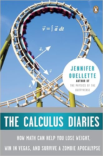
Kiss My Math meets A journey of the Calculus
Jennifer Ouellette by no means took math in university, generally simply because she-like such a lot people-assumed that she wouldn't want it in actual lifestyles. yet then the English-major-turned-award-winning-science-writer had a metamorphosis of middle and made up our minds to revisit the equations and formulation that had haunted her for years. The Calculus Diaries is the thrill and engaging account of her yr spent confronting her math phobia head on. With wit and verve, Ouellette exhibits how she realized to use calculus to every little thing from fuel mileage to weight loss plan, from the rides at Disneyland to taking pictures craps in Vegas-proving that even the mathematically challenged can examine the basics of the common language.
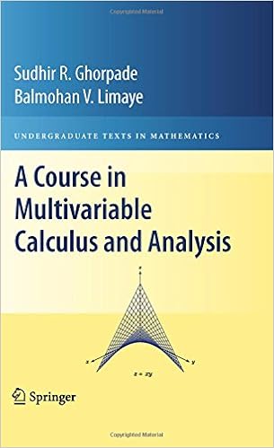
A Course in Multivariable Calculus and Analysis (Undergraduate Texts in Mathematics)
This self-contained textbook supplies an intensive exposition of multivariable calculus. it may be considered as a sequel to the one-variable calculus textual content, A path in Calculus and genuine research, released within the related sequence. The emphasis is on correlating basic recommendations and result of multivariable calculus with their opposite numbers in one-variable calculus.
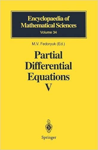
The six articles during this EMS quantity offer an outline of a couple of modern recommendations within the research of the asymptotic habit of partial differential equations. those ideas contain the Maslov canonical operator, semiclassical asymptotics of suggestions and eigenfunctions, habit of options close to singular issues of other varieties, matching of asymptotic expansions on the subject of a boundary layer, and approaches in inhomogeneous media.
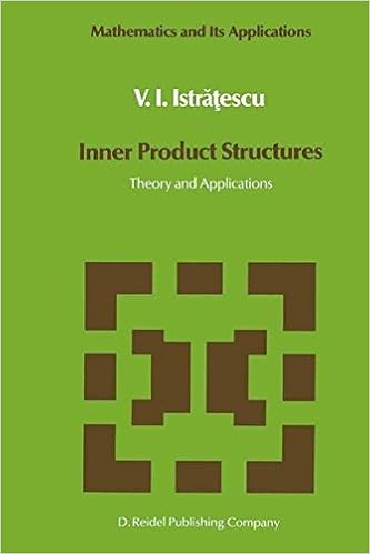
Inner Product Structures: Theory and Applications
Process your difficulties from the appropriate finish it is not that they cannot see the answer. it truly is and start with the solutions. Then in the future, that they can not see the matter. maybe you can find the ultimate query. G. ok. Chesterton. The Scandal of dad 'The Hermit Oad in Crane Feathers' in R. Brown 'The aspect of a Pin'.
- Lebesgue Measure and Integration: An Introduction
- Matrix Methods in Analysis
- Singular Integral Operators
- A First Course in Integral Equations
- Itô’s Stochastic Calculus and Probability Theory
Extra resources for Microcomputer Modelling by Finite Differences
Example text
All of which gives us the next program. Program 7 (Suitable as listed for the IBM PC or the Apple II) 100 200 300 400 500 999 GOSUB GOSUB GOSUB GOSUB GOSUB STOP 1000: 2000: 3000: 4000: 5000: REM REM REM REM REM INITIALISE SET UP PROBLEM BOUNDARY CONDITIONS SOLVE THE PROBLEM PRINT THE SOLUTION 1000 REM SUBROUTINE FOR INITIALISATION 1010 DIM X(20),Y(20) 1015 DIM A(20),B(20),C(20),D(20) 1020 INPUT "NUMBER OF NODES "iN 1030 INPUT "LENGTH OF DOMAIN "iL 1040 DX = L / (N - 1): REM INTERVAL BETWEEN NODES 1050 REM CALCULATE THE GRID 1060 X(l) = 0 1070 FOR I = 2 TO N 38 Microcomputer Modelling by Finite Differences 1080 XII) = XII - 1) + OX 1090 NEXT I 1100 C3 = 0: REM INITIALISE THE COUNTER C3 1999 RETURN 2000 REM SUBROUTINE FOR THE PHYSICAL PROPERTIES 2010 DEF FN F(X) = 2 2020 INPUT "ENTER A fIlA 2030 INPUT "ENTER B "lB 2040 INPUT "ENTER C "lC 2100 REM CALCULATE G1,G2 AND G4 2110 G1 = - B / 2 / OX - A / OX / OX 2120 G2 = B / 2 / OX - A / OX / DX 2130 G4 = C - 2 * A / OX / OX 2999 RETURN 3000 3010 3020 3030 3999 REM SUBROUTINE FOR SETTING BOUNDARY CONDITIONS INPUT "Y(l) "lY(l) PRINT "VALUE OF Y AT X="lLl INPUT YIN) RETURN 4000 REM SUBROUTINE FOR CALCULATING THE SOLUTION 4010 REM CALCULATE THE Y'S 4015 D3 = 0: REM SET RESIDUAL TO ZERO 4020 FOR I = 2 TO N - 1: REM ONLY TO N-1 NOW!!
Before doing this, fmd out where the RESET or BREAK button is on your computer. Why? 1 should suggest to you that we ought really to be looking at fractional rather than absolute changes. In line 4035 of Program 4 we simply add up the absolute values of the differences between the old and the new values of the dependent variables at each node. This could be improved by replacing line 4035 by a line such as 4035 03=03 + AB5(O-Y(I»/AB5(O + 1E-6) This change will ensure that the values of the residual are 'normalised' before we use them.
But we shall not be using vectors any more, so it does not matter if you have never used the shorthand of vector operators. 1) written out in full for cartesian coordinates in two dimensions is then ~ ax (k axaT) + ~(k ay aT) ay You will often see this simplified to k(aaxT + a T) 2 ay2 2 2 but this form is true only if k is constant in space - that is, if it does not change its value from point to point. 1) is to allow for varying values of k, so we shall use the slightly more complicated form for the left-hand side of the equation.