By Anatoli Torokhti, Phil Howlett
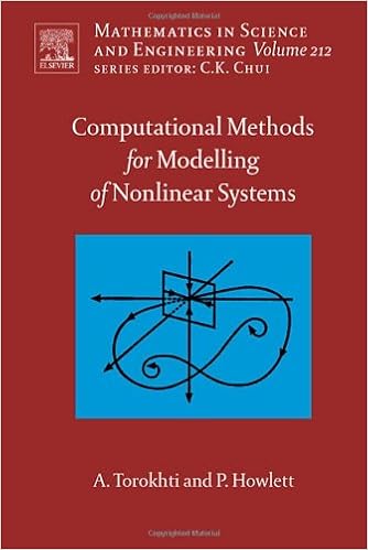
In this booklet, we research theoretical and useful elements of computing tools for mathematical modelling of nonlinear structures. a few computing concepts are thought of, corresponding to equipment of operator approximation with any given accuracy; operator interpolation strategies together with a non-Lagrange interpolation; tools of process illustration topic to constraints linked to ideas of causality, reminiscence and stationarity; tools of procedure illustration with an accuracy that's the top inside of a given category of versions; equipment of covariance matrix estimation; equipment for low-rank matrix approximations; hybrid equipment in accordance with a mixture of iterative techniques and most sensible operator approximation; and techniques for info compression and filtering less than situation clear out version should still fulfill regulations linked to causality and sorts of memory.
As a end result, the ebook represents a mix of recent tools commonly computational research, and particular, but additionally familiar, suggestions for examine of structures conception ant its specific branches, resembling optimum filtering and data compression.
- Best operator approximation
- Non-Lagrange interpolation
- Generic Karhunen-Loeve transform
- Generalised low-rank matrix approximation
- Optimal information compression
- Optimal nonlinear filtering
Read or Download Computational Methods for Modeling of Nonlinear Systems, Vol. 1 PDF
Similar linear books

Lie Groups Beyond an Introduction
This ebook takes the reader from the tip of introductory Lie crew thought to the brink of infinite-dimensional workforce representations. Merging algebra and research all through, the writer makes use of Lie-theoretic tips on how to enhance a stunning conception having vast functions in arithmetic and physics. The publication at the beginning stocks insights that utilize genuine matrices; it later depends on such structural positive aspects as homes of root structures.
Lectures on Tensor Categories and Modular Functors
This ebook supplies an exposition of the kinfolk one of the following 3 themes: monoidal tensor different types (such as a class of representations of a quantum group), three-d topological quantum box conception, and 2-dimensional modular functors (which certainly come up in 2-dimensional conformal box theory).
We improve the speculation of compactness of maps among toposes, including linked notions of separatedness. This thought is equipped round types of 'propriety' for topos maps, brought the following in a parallel type. the 1st, giving what we easily name 'proper' maps, is a comparatively susceptible as a result of Johnstone.
- Stability of Linear Systems: Some Aspects of Kinematic Similarity
- Lie Algebras, Finite and Infinite Dimensional Lie Algebras and Applications in Physics, Part 1
- Linear Algebraic Monoids
- Mathematik für Ingenieure: Eine anschauliche Einführung für das praxisorientierte Studium
Additional info for Computational Methods for Modeling of Nonlinear Systems, Vol. 1
Example text
Definition 1 A solution to (1) is a set of n scalars x1 , x2 , . . , xn that when substituted into (1) satisfies the given equations (that is, the equalities are valid). System (1) is a generalization of systems considered earlier in that m can differ from n. If m > n, the system has more equations than unknowns. If m < n, the system has more unknowns than equations. If m = n, the system has as many unknowns as equations. 3 may be used to convert (1) into the matrix form Ax = b, (2) 43 44 Chapter 2 where Simultaneous Linear Equations ⎡ ⎤ a1n a2n ⎥ ⎥ ..
Prove that if a 2 × 2 matrix A commutes with every 2 × 2 diagonal matrix, then A must also be diagonal. Hint: Consider, in particular, the diagonal matrix D= 1 0 0 . 0 18. Prove that if an n × n matrix A commutes with every n × n diagonal matrix, then A must also be diagonal. 19. Compute D2 and D3 for the matrix D defined in Problem 15. 20. Find A3 if ⎡ 1 A = ⎣0 0 0 2 0 ⎤ 0 0⎦. 3 21. Using the results of Problems 19 and 20 as a guide, what can be said about Dn if D is a diagonal matrix and n is a positive integer?
Example 1 Graph the vectors v = [2 magnitude and angle of each. 5. 4◦ . 1 = −1, and −1 θ = 135◦ . 14, tan θ = To construct the sum of two vectors u + v geometrically, graph u normally, translate v so that its initial point coincides with the terminal point of u, being careful to preserve both the magnitude and direction of v, and then draw an arrow from the origin to the terminal point of v after translation. 6 represents the sum u + v. 6 for the two vectors defined in Example 1. To construct the difference of two vectors u − v geometrically, graph both u and v normally and construct an arrow from the terminal point of v to the terminal point of u.